Comprehensive RNA-Seq Data Analysis: From Gene to Transcript Level

Syllabus Overview

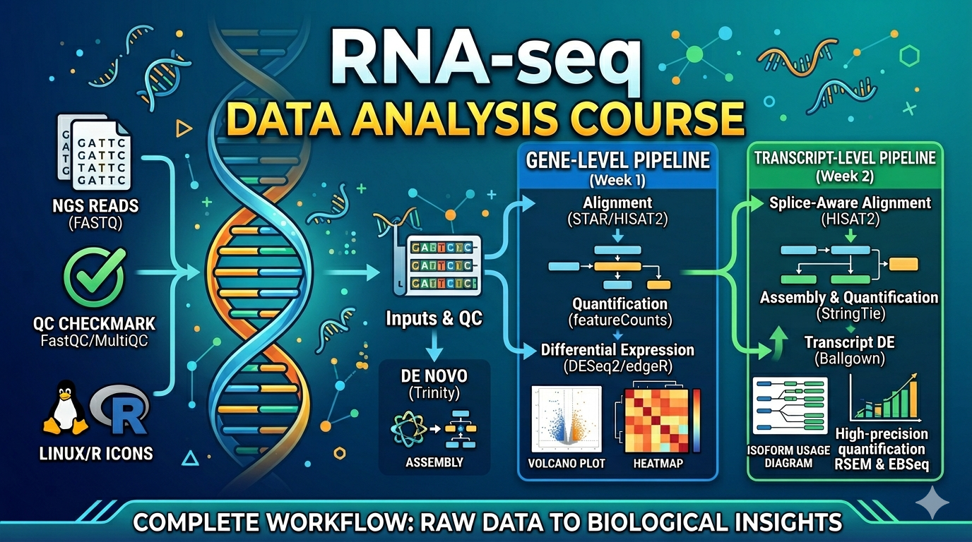
Week 1 — RNA-Seq Data Analysis (Gene-Level Pipeline)

Class 1: Introduction to NGS & NGS Data Types

Objective: Understand NGS technologies, applications, and data formats

• What is NGS? Sequencing platforms (Illumina, ONT, PacBio)

• Applications: Genomics, Transcriptomics, Metagenomics, Epigenomics

• NGS workflow overview

• Infrastructure requirements for NGS data analysis

• NCBI SRA/ENA/GEO databases, metadata understanding

Hands-on:

• Linux basics (navigation, permissions, pipes, grep, awk)

• Navigate NCBI SRA, ENA

• Using SRA Toolkit: prefetch, fasterq-dump

• Download sample datasets manually

Class 2: Introduction to RNA-seq & Experimental Design

Objective: Understand RNA-seq fundamentals and experimental design

• Overview of RNA-seq: concepts, applications, and data generation

• Bulk RNA-seq vs single-cell RNA-seq

• Library types: PolyA vs rRNA depletion, stranded vs unstranded

• Replicates: biological vs technical

• Sequencing depth and batch effects

Hands-on:

• Download RNA-seq publicly available dataset

• Inspect metadata and study design

Class 3: RNA-seq QC & Preprocessing

Objective: Perform QC & trimming for transcriptomics data

• FASTQ structure and quality metrics

• Quality assessment tools: FastQC, fastp, MultiQC

• Key QC parameters: adapters, duplication rate, GC content, overrepresented sequences

• Adapter and quality trimming concepts

Hands-on:

• Run FastQC and MultiQC

• Trim reads using Trimmomatic / fastp / Trim Galore

• Post-QC evaluation

Class 4: Alignment & Gene Quantification

Objective: Map reads and generate gene-level counts

• Alignment algorithms: HISAT2, STAR

• Genome indexing and mapping concepts

• SAM/BAM file basics

• Gene quantification methods: featureCounts, HTSeq

Hands-on:

• Perform alignment using HISAT2 / STAR

• (Optional exposure) Run pseudo-alignment using Salmon / Kallisto

• Convert SAM to BAM, sorting & indexing (samtools)

• Generate gene-level count matrix using featureCounts / HTSeq

Class 5: Differential Expression & Functional Analysis (Gene-Level)

Objective: Identify DEGs and biological interpretation

• Concept of differential gene expression

• Normalization methods (counts vs TPM/FPKM)

• Tools: DESeq2, edgeR, limma-voom

• Visualization: volcano plot, heatmap

• Functional analysis: GO, KEGG pathways

Hands-on:

• Perform DEG analysis using DESeq2 / edgeR / limma

• Generate volcano plot and heatmap

• Perform GO/KEGG pathway analysis

Class 6: De Novo Transcriptome Assembly & Annotation

Objective: Assemble and quantify a transcriptome for organisms without a reference genome.

De Novo Concepts: Challenges of assembling short reads without a reference; the De Bruijn Graph approach.

Trinity Workflow: Inchworm, Chrysalis, and Butterfly modules for full-length transcript reconstruction.

Transcript Clustering: Reducing redundancy in raw assemblies using CD-HIT.

Quantification: High-speed transcript abundance estimation using Kallisto (pseudo-alignment).

Functional Annotation: Overview of identifying open reading frames (TransDecoder) and BLAST searching.

Hands-on:

·      Perform de novo assembly using Trinity from raw FASTQ files.

·      Cluster sequences with CD-HIT to generate a non-redundant set.

·      Assess assembly quality (ExN50 metrics and BUSCO).

·      Map reads back to the assembly using Kallisto to generate count matrices.

·      Basic functional annotation using BLAST against a known protein database.

Week 2 — HISAT2–StringTie–Ballgown Pipeline (transcript level pipeline)

Class 7: Introduction to Transcript Assembly & Pipeline Overview

Objective: Understand transcript-level pipeline and workflow

• Limitations of gene-level analysis

• Concept of transcript assembly and isoforms

• Overview of HISAT2 → StringTie → Ballgown pipeline

• Reference-guided transcript assembly

• GTF files and transcript annotations

Hands-on:

• Prepare reference genome and annotation files

• Build HISAT2 index

• Understand pipeline structure

Class 8: Alignment using HISAT2

Objective: Perform splice-aware alignment for transcript assembly

• HISAT2 alignment strategy

• Handling paired-end vs single-end reads

• Output formats (SAM/BAM)

• Importance of sorted BAM for downstream analysis

Hands-on:

• Align reads using HISAT2

• Convert, sort, and index BAM files using samtools

• View BAM files in IGV viewer, so view splice junctions & split reads

Class 9: Transcript Assembly & Quantification using StringTie

Objective: Assemble transcripts and estimate abundance

• Transcript assembly concepts

• StringTie workflow

• Expression metrics: RPKM, FPKM, TPM

• Merging transcripts across samples

Hands-on:

• Run StringTie for transcript assembly

• Generate GTF files

• Merge transcripts using StringTie --merge

Class 10: Differential Expression using Ballgown

Objective: Perform transcript-level differential expression

• Ballgown workflow

• Importing StringTie output into R

• Statistical modeling for transcript expression

• Visualization and interpretation

Hands-on:

• Prepare Ballgown input files

• Perform differential expression analysis using Ballgown

• Extract significant transcripts

Class 11: Advanced Interpretation & Visualization

Objective: Interpret transcript-level results and compare with gene-level

• Isoform-level expression patterns

• Differential transcript usage concepts

• Comparing gene-level vs transcript-level results

• Biological interpretation of isoform changes

Hands-on:

• Visualize transcript expression changes

• Compare gene vs transcript results

• Prepare final report and summary

Class 12: High-Precision Quantification with RSEM & EBSeq

Objective: Perform EM-based isoform quantification and differential expression analysis.

RSEM Logic: Multi-mapping reads and the Expectation-Maximization (EM) algorithm.

The Workflow: Reference indexing, abundance estimation, and "Expected Counts" vs. TPM.

Differential Expression with EBSeq: Handling isoform-level uncertainty and Bayesian posterior probabilities.

Hands-on:

·      Build RSEM indices and run rsem-calculate-expression from FASTQ/BAM.

·      Generate gene/isoform count matrices.

·      Run EBSeq in R to identify differentially expressed transcripts.

·      Compare RSEM results with gene-level (Week 1) and assembly-based (Week 2) outputs